#data visulaization
Explore tagged Tumblr posts
Visit Tumblr Blog
Explore Tumblr blogs with no restrictions, modern design and the best experience.
Last Seen Tumblr Blogs


Fun Fact
Tumblr posted its first advertisements in May 2012 and subsequently earned $13M in revenue.
Text

Jupyter Notebook Integration of g.nome
The integration of data visualization through Jupyter Notebook significantly enhances the capabilities of g.nome, streamlining the iterative process. This integration enables seamless processing and visualization of reciprocal file sharing, facilitating the exploration of data crucial for the advancement of modern medicine. Additionally, users have the flexibility to record notes and interpret analyses in a fully customizable format, empowering them to tailor their workflow to their specific needs and preferences.
0 notes
Text
Price: [price_with_discount] (as of [price_update_date] - Details) [ad_1] From the manufacturer Designed to Charge Fast 10x Data Transfer Speed UH700 can deliver up to 5V/1.5A output that charges 50% faster and saves up to 30% on charging time*. Fully charging a Galaxy S6 edge takes just 100 minutes with the UH700 USB Hub, whereas it takes 150 minutes with a USB Hub supporting 5V/1A output. Equipped with USB 3.0 ports, the UH700 can transfer a 1080p movie under 2 minutes 18 seconds, whereas it takes 7 minutes 36 seconds with a USB Hub equipped with USB 2.0 ports.* *The actual transmission speed depends on the setting of the device connected. 7 data transfer ports mean you don't have to switch between devices Increase the number of available ports The UH700 is perfect for anyone who has a computer with only one or two USB ports, and wants easier access toadditional ports without having to switch between devices. Considerate Design A dim white LED indicator on the power button helps visulaize the connection status and similarly 7 dim white LED indicators beyond each USB port also indicate whether the devices are properly connected. Protect Both Your Devices and Precious Data UH700 has a sophisticated circuit design with multiple protections for your devices against over-heating, over-current, over-voltage and short circuit. A built-in surge protector keeps both your devices and data safe in the process of transferring data. UH700 support USB ports hot swapping that can be safely connected and disconnected while the computer is powered on and running. Short circuit Over-voltage Over-current Over-heating USB 3.0 —— USB 3.0 ports offer transfer speeds of up to 5Gbps, 10 times faster than standard USB 2.0 10 x Data Transfer Speed —— The 7 data transfer ports mean you don't have to switch between devices Charge Fast —— UH700 can deliver up to 5V/1.5A output that charges 50% faster and saves up to 30% on charging time Output Interface —— 7 USB 3.0 Standard A Input Interface —— 1 USB 3.0 Micro B Compatibility —— Windows, Mac OS X and Linux systems Chipset —— RTS5411 Worry-free customer support —— For other installation related query, compatibility issue or any other queries call on toll free no 1800 2094 168 or write us at [email protected]
0 notes
Photo
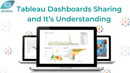
Visit: https://medium.com/@jhones1998olivia/tableau-dashboards-sharing-and-its-understanding-905506549862
Tableau Dashboards Sharing and Its Understanding
Creating or planning a dashboard isn't just about putting representation components that are presented by Tableau. A dashboard ought to have the most important data that is reasonable for speedy utilization of data by a client. Tableau gives plenty of instruments to intuitiveness including tooltips and channels/filters, making utilization of them without jumbling the visible region will prompt a lovely dashboard experience.
0 notes
Video
youtube
Kersey Sturdivant and I were lucky enough to share the TEDx stage here in Newport, RI. We discussed life in the seafloor, how we know about it, and the efforts we’ve undertaken with INSPIRE Environmental to visualize this cryptic environment.
#Three.js#Science#Benthos#SPI#Sediment#Sediment Profile Imaging#Ocean#Marine#Biology#3D#Computer Graphics#Data Visulaization#Newport#Rhode Island#TEDx#INSPIRE Environmental
0 notes
Text
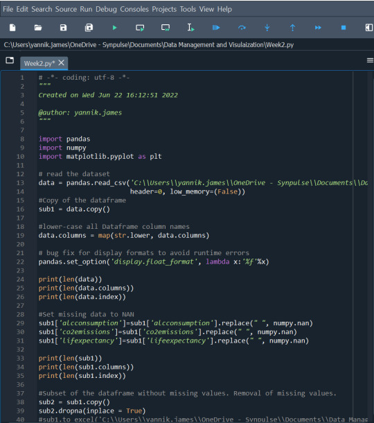
Week 3: Peer Graded Assignment (Data Management and Visualization)
Program
import pandas import numpy import matplotlib.pyplot as plt
#read the dataset
data = pandas.read_csv('C:\Users\yannik.james\OneDrive - Synpulse\Documents\Data Management and Visulaization\Data Sets\gapminder1.csv', header=0, low_memory=(False))
#Copy of the dataframe
sub1 = data.copy()
#lower-case all Dataframe column names
data.columns = map(str.lower, data.columns)
#bug fix for display formats to avoid runtime errors
pandas.set_option('display.float_format', lambda x:'%f'%x)
print(len(data)) print(len(data.columns)) print(len(data.index))
#Set missing data to NAN
sub1['alcconsumption']=sub1['alcconsumption'].replace(" ", numpy.nan) sub1['co2emissions']=sub1['co2emissions'].replace(" ", numpy.nan) sub1['lifexpectancy']=sub1['lifeexpectancy'].replace(" ", numpy.nan)
print(len(sub1)) print(len(sub1.columns)) print(len(sub1.index))
#Subset of the dataframe without missing values. Removal of #missing values.
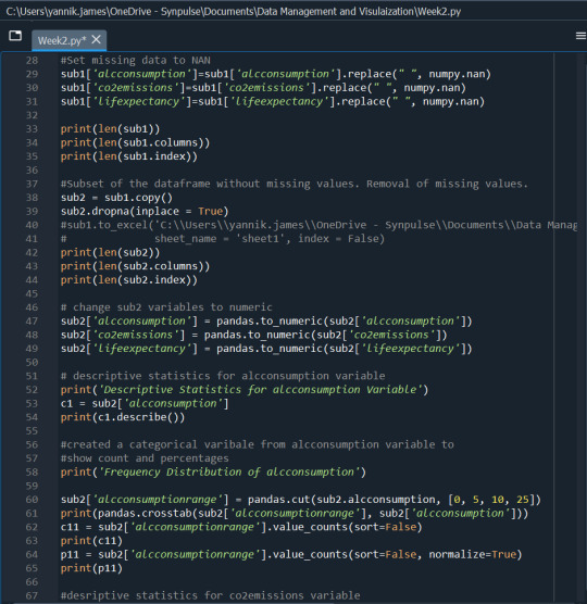
sub2 = sub1.copy() sub2.dropna(inplace = True)
print(len(sub2)) print(len(sub2.columns)) print(len(sub2.index))
#change sub2 variables to numeric
sub2['alcconsumption'] = pandas.to_numeric(sub2['alcconsumption']) sub2['co2emissions'] = pandas.to_numeric(sub2['co2emissions']) sub2['lifeexpectancy'] = pandas.to_numeric(sub2['lifeexpectancy'])
#descriptive statistics for alcconsumption variable
print('Descriptive Statistics for alcconsumption Variable') c1 = sub2['alcconsumption'] print(c1.describe())
#created a categorical varibale from alcconsumption variable to #show count and percentages
print('Frequency Distribution of alcconsumption')
sub2['alcconsumptionrange'] = pandas.cut(sub2.alcconsumption, [0, 5, 10, 25]) print(pandas.crosstab(sub2['alcconsumptionrange'], sub2['alcconsumption'])) c11 = sub2['alcconsumptionrange'].value_counts(sort=False) print(c11) p11 = sub2['alcconsumptionrange'].value_counts(sort=False, normalize=True) print(p11)
#desriptive statistics for co2emissions variable
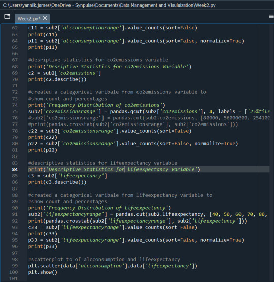
print('Desriptive Statistics for co2emissions Variable') c2 = sub2['co2emissions'] print(c2.describe())
#created a categorical varibale from co2emissions variable to show #count and percentages
···
print('Frequency Distribution of co2emissions') sub2['co2emissionsrange'] = pandas.qcut(sub2['co2emissions'], 4, labels = ['25%tile','50%tile','75%tile','100%tile'])
print(pandas.crosstab(sub2['co2emissionsrange'], sub2['co2emissions']))
c22 = sub2['co2emissionsrange'].value_counts(sort=False) print(c22) p22 = sub2['co2emissionsrange'].value_counts(sort=False, normalize=True) print(p22)
#descriptive statistics for lifeexpectancy variable
print('Descriptive Statistics for lifeexpectancy Variable') c3 = sub2['lifeexpectancy'] print(c3.describe())
#created a categorical varibale from lifeexpectancy variable to #show count and percentages
print('Frequency Distribution of lifeexpectancy') sub2['lifeexpectancyrange'] = pandas.cut(sub2.lifeexpectancy, [40, 50, 60, 70, 80, 90]) print(pandas.crosstab(sub2['lifeexpectancyrange'], sub2['lifeexpectancy'])) c33 = sub2['lifeexpectancyrange'].value_counts(sort=False) print(c33) p33 = sub2['lifeexpectancyrange'].value_counts(sort=False, normalize=True) print(p33)
Summary
The three variables I have chosen, alcconsumption, co2emissions and lifeexpectancy, are all continuous variables. The two main data management techniques I utilized for this dataset was grouping/ binning and dealing with missing values. Since the data was continuous, I had to group the data for each variable in order to create their frequency distributions. I also created a summary of their descriptive statistics summary.
For the variable alcconsumption, it was divided into three groups. Most countries fell in the “0-5” category, then the second most fell in the “5-10” category and the least prominent group was the “10-25” group which were countries with a reading over 10. The average reading was 6.63.
Second for co2emissions, I found that the highest emission was 334000000000 and the lowest was 850666.67. The mean was recorded at 5774913036.826859 and the median was 254030333.3. There were a few outliers that were significantly higher than the rest of the countries causing the stark difference between the mean and medium calculation. I also grouped this variable in percentiles; 25th, 50th, 75th and 100th percentile. There were 43 data points in each group, thus each group contains 25% of the total datapoints.
Third for lifeexpectancy, I grouped them just like alcconsumption. This time into 5 categories; less than 50, 50-60, 60-70, 70-80 and greater than 80. The 70-80 category had the highest frequency, followed by 60-70, then 50-60, then greater than 80 and finally less than 50.
As I said previously, apart from grouping, another data management technique I utilized was to deal with the missing values in my variables. All three variables above each had missing data and to deal with this, I removed rows with missing data. Since it was not that many rows, removing some row still kept the integrity of the dataset.
0 notes
Text
Top 10 SEO tools to grow your website
Search Engine Optimization is an integral part of growing your website. Your brand needs a flexible and intuitive SEO strategy for keeping up with the competitors. The algorithms of Search engines change constantly. SEO tools can help you cope up with the changes and offer data like keyword targeting, link building techniques and competitor's analysis. You can avail SEO services from the top digital marketing companies in Indore.
If you're wondering as to how these tools can help you, here's your answer. Smart tools will enhance your workflow and productivity. The right tools will save your time and efforts. There are several tools available at your disposal. We have researched and picked up the perfect fits which are a must have for every brand.
Top 10 SEO Tools
Google Analytics
This tool will help you to get a complete idea of the website, including web statistics and search insights. It tracks all the traffic on your website for a detailed report. You can get a list of mostly searched keywords which will help users land on your webpages.
To get keywords, go to Acquisition > Search Console > Queries > Campaigns > Organic Keywords
Alternatives to Google Analytics are Matomo, Click and Open Web Analytics.
SEMrush
SEMrush is one of the most useful tools for SEO. It primarily focuses on researching keywords and keyword phrases. With a database of 35 million keywords, it is the perfect tool for finding target keywords to rank higher than your competitors. You can get in touch with top SEO companies in Indore to get professional assistance.
It shows a detailed report including:
Keyword volume
CPC (average cost per click)
Competitive Density
KD (ranking difficulty)
Trends over the past months
Snapshot of the result
Various websites that rank for it
Broken Link Checker
Broken Link Checker is a free tool which will help you find broken links. Having several broken links will decrease the traffic to your website. You will start losing audience. Finding such links individually can be a cumbersome task. This tool will scan individual pages and the complete website for finding such links. The broken links will be highlighted in the report.
Google Data Studio
When it comes to LSEO, Google Data Studio is mandatory. Since reporting can prove to be dynamic and stressful, this tool makes the process easier. Set up the metrics for tracking and it will do the rest automatically. It supports several connectors which will let you gather data from almost every resource. Doing this on your own can be confusing. We recommend that you avail SEO services from top SEO companies in Indore.
Yoast
Yoast is another crucial SEO tool which does magic to your Wordpress site. It has an audit tool for deeply checking the website. You can choose from several SEO review options. The packages depend on the pricing and the level of Yoast you require. For example: The starting package is the Silver SEO review for $699 followed by Diamond Review.
Exploding Topics
Do you wish to find target keywords before your competitors? Exploding Topics is the perfect keyword for this. It will offer information about the topics which are just starting to trend. The bubble visulas add aesthetics to the tool. You can develop content around these newly trending topics for increased visibility and reach in near future. You will find an option called ‘Categories’, which will help you shortlist your niche for getting an efficient report.
SEO Optimer
If you are looking for a tool which will check your website, have an overall look and offer feedback, here’s your best fit. SEO Optimer conducts a deep check of your complete website under 30 seconds. It offers scores for on-page factors. You will find a few recommendations for making the process smooth. You can get in touch with the best SEO companies in Indore like Hype Digitally for professional assistance.
AnswerThePublic
Get a list of the frequently searched questions by the users on various search engines. Who knew this would be possible? AnswerThePublic is a frivolous tool which will offer you valuable data, as to what topics you should focus on. This will increase your reach and bring more traffic to your website. If you use the tool the right way, you may just hit a jackpot. The top digital marketing companies in Indore use this tool for enhanced performance.
Google Pagespeed Insights
This tool will let you know the speed of your website and usability on different devices. All you need to do is Enter a URL and the tool will do the rest. It will tell your minor details like page loading time and performance for desktop and mobile phones. Get more information like performance score and grading areas.
Mangools
Mangools offers you with a phenomenal cloud-based tool suite. It includes SERPChecker, SiteProfile, SERPWatcher, KWFinder and LinkMiner. Many SEO agencies in Indore approve these tools as a cost-effective option for added efficiency.
Conclusion
There are several SEO tools to help you out with the process. We have listed the ones utilised by the top SEO agencies in Indore. Hype Digitally is one of the best Digital Marketing companies in Indore. We use the latest tools and technologies to offer brands with the best results. Grow and expand your business empire. If you are looking for SEO services from an expert team, we are eager to assist you. Get in touch now!
#seo services#seo agency seo marketing company#search engine optimization company in indore#seo company in indore#best seo company in indore#seo services indore#seo companies in indore#seo agency in indore#SEO in indore#Top digital marketing companies in indore
0 notes
Photo

Hey all, We are looking for an atleast 2 years of experience Fornt-end UI Designer. Salary negotiable for suitable candidates. Required urgently and for long term basis. Please send your resume to [email protected] or call at +91-9409394242 Fornt-end UI Designer (1 position) Experience: - 2-3 years of experience in Web applications design and development. - Excellent knowledge of Html, CSS, JavaScript, jquery, Bootstrap (all versions) - Excellent knowledge on data visulaization tool D3.JS - Working experience on React JS or Angular JS (version 2 and above) - Good knowledge of Client-Server Architecture, network communication and good designing principles. - Basic web and mobile apps design experience (UI elements, Icons etc.,) - Ability to write well-documented and maintainable JS code. - Familiarity with git - Test websites across multi-browser configurations and identify any issues - Strong interpersonal skills and demonstrated the ability to build professional relationships. - Excellent Problem solving skills with innovative and proactive approach. - Proficient in debugging and fixing bugs in minimal time - Ability to work individually and in a team. #frontenddeveloper #jobopenings #hiringnow #recruitment #vadodarahr #vadodara_lover #uideveloper https://ift.tt/2J9zSiF
0 notes
Text
Data Management and Visualization - Week 2
# -*- coding: utf-8 -*- """ Created on Sat Nov 3 19:38:53 2018
@author: Janani """
import numpy as np import matplotlib.pyplot as plt import pandas as pan from sklearn.cross_validation import train_test_split from sklearn.tree import DecisionTreeClassifier from sklearn.metrics import classification_report import sklearn.metrics from io import BytesIO as StringIO from sklearn import datasets import math from pylab import * import seaborn as sb
#reading the first data data= pan.read_csv("C:/Users/Janani/Desktop/Imp - DS/My Southampton/Data Visulaization/Data/Data Final/Women-API-Enroll.csv") #structure of data data.dtypes data.shape (111, 48)
#columns in dataset data.columns
['Country ID', 'Region 1 - ID', 'Region 1 - Enroll', 'Region 2', 'Income Group', 'Country', '1970', '1971', '1972', '1973', '1974', '1975', '1976', '1977', '1978', '1979', '1980', '1981', '1982', '1983', '1984', '1985', '1986', '1987', '1988', '1989', '1990', '1991', '1992', '1993', '1994', '1995', '1996', '1997', '1998', '1999', '2000', '2001', '2002', '2003', '2004', '2005', '2006', '2007', '2008', '2009', '2010', 'Unnamed: 47'], dtype='object')
#describe data data.describe() 1970 1971 ... 2010 Unnamed: 47 count 111.000000 111.000000 ... 111.000000 0.0 mean 1.963964 3.094595 ... 18.768468 NaN std 4.928337 6.118271 ... 11.076478 NaN min 0.000000 0.000000 ... 0.000000 NaN 25% 0.000000 0.000000 ... 10.650000 NaN 50% 0.000000 0.000000 ... 16.800000 NaN 75% 1.550000 3.600000 ... 25.400000 NaN max 30.500000 30.500000 ... 45.000000 NaN data.info()
#check for missing data data.isnull().sum() data.columns.isnull().any()
data['Country'].describe() count 111 unique 111 top Canada freq 1 Name: Country, dtype: object
print("How many Income Groups the countries are categorized into?") print(data['Income Group'].value_counts(sort = False))
Lower middle income 24 Upper middle income 32 High income 37 Low income 18
print("How many Regions the countries are categorized into?") print(data['Region 1 - Enroll'].value_counts(sort = False))
Eastern Europe 8 Asia and the Pacific 16 Middle East and North Africa 13 Sub-Saharan Africa 24 Latin America and the Caribbean 26 Advanced Economies 24
#reading the first data data_2= pan.read_csv("Enroll - 1970 - 2010.csv") #structure of data data_2.dtypes data_2.shape
(999, 17)
#columns in dataset data_2.columns
Index(['Country ID', 'Country', 'Year', 'No Schooling', 'Primary - Enrolled', 'Primary - Attained', 'Secondary - Enrolled', 'Secondary - Attained', 'Tertiary - Enrolled', 'Tertiary - Attained', 'Avg. Years of Total Schooling', 'Avg. Years of Primary Schooling', 'Avg. Years of Secondary Schooling', 'Avg. Years of Tertiary\n Schooling', 'Population\n(1000s)', 'Region', 'Region ID'], dtype='object')
print("What are the conutries where the 'Primary - Attained' is greater than 60%?") a = (data_2['Country'][data_2['Primary - Attained']>60.0 ]) print(a.unique().tolist())
What are the conutries where the 'Primary - Attained' is greater than 20%? Country Code Country 145 Norway 387 Hungary 450 Belize
There are only three countries out of the whole set to have atleast 60% of female who attained Primary Education
print("What are the Countries where the 'Tertiary - Attained' is greater than 30%?") print(data_2['Country'][data_2['Tertiary - Attained']>30.0].unique().tolist())
What are the Countries where the 'Tertiary - Attained' is greater than 30%? Country Code Country 35 Canada 80 Greece 98 Ireland 205 USA 332 Korea, North 341 Korea, South There are only six countries out of the whole set to have atleast 30% of female who attained Tertiary Education between 1970 to 2010 which is very alarming.
print("What are the Regions where the 'Secondary - Attained' is greater than 40%?") a = (data_2['Region'][data_2['Secondary - Attained']>40.0 ]) print(a.unique().tolist())
What are the Regions where the 'Secondary - Attained' is greater than 40%?
Region
Advanced Economies Asia and the Pacific Eastern Europe Latin America the Caribbean Sub-Saharan Africa
If we take count Region wise then the above regions have atleast 40% of
female who attained Secondary Education between 1970 to 2010.
0 notes
Text
Elasticsearch 6.0: Learn Elasticsearch, Kibana from Scratch
http://bit.ly/2GmrslN Elasticsearch 6.0: Learn Elasticsearch, Kibana from Scratch, Learn Elasticsearch & Kibana from scratch, Store, Search, Visulaize & Analyze Big Data on cluster with Elasticsearch.
0 notes
Text
BIG DATA
기업에 축적된 데이터를 분석하기 위해 데이터 웨어하우스와 데이터 마이닝이 90년대말, 활발히 도입되었다.
빅데이터란 Volume-Variety-Velocity의 3가지 특성으로 정의된다.
데이터 과학이란 통계학과 컴퓨터 과학 등 다양한 학문과 기술이 융합된 것이다.
빅데이터 시대에 필요한 기술 : 분산처리 기반의 데이터 가공 및 컴퓨터기술, 데이터 시각화, 실시간 대응을 위한 관련 기술
인공지능 - IBM의 왓슨은 미국의 퀴즈프로에서 우승을 한바 있다, 인공지능은 자연어처리 및 인식 등에 활용된다, 딥러닝이라는 알고리즘이 전 세계의 관심을 받고 있다.
SNS기반의 연결된 사회 - 페이스북(facebook)은 친구들 혹은 같은 관심을 갖는 사람들을 연결해 준다, 트위터(tweeter)는 연결된 사람 혹은 기업들 간을 연결하여 소통을 가능하게 해 준다, 링크드인(linked-in)은 개인의 이력을 중심으로 전문가들 간의 관계망을 형성한다. 건전한 사회 실현을 위해 데이터 과학자가 하여할 일과 관련된 것은 자금세탁방지, 보험사기방지, 품질보증사기탐색
빅데이터 시대에 필요한 분석기술은 과거의 데이터 분석기술과 차별화된다.
데이터 과학자는 통계학이나 IT지식 외에 소통능력이나 시각화와 관련된 디자인 능력 등 다방면의 능력이 요구된다.
빅데이터 기반 학습 알고리즘으로 인공지능은 비약적으로 발전하고 있다.
새로운 개념의 협업 필터링 알고리즘을 탄생시킨 넷플릭�� 경진대회는 데이터 과학자의 중요성을 알리는 계기가 되었다.
구글의 검색어 데이터를 활용하여 각종 예측이 가능하다.
착용 가능한 센서를 통해 건강관련 데이터를 모으고 분석하여 인간의 삶의 질을 향상시킬 수 있다.
데이터 과학자는 다양한 사기 등을 방지 혹은 탐지할 수 있다.
빅데이터는 데이터의 크기가 크고 형태가 비정형화 되어 있으며, 생성속도가 빠른 데이터이다.
빅데이터 분석을 통해 새롭게 ���아내는 지식의 양은 적지만, 이를 통한 파급효과는 크다.
빅데이터 이용시 문제가 될 수 있는 부분이 사생활 침해와 관련된 문제들이 있다. 유럽과 미국정부에서 개인정보 이용 시 개인의 동의가 반드시 필요한 법률체계를 옵트인(Opt in)이라고 부른다.
옵트인 방식은 개인에게 개인정보 수집에 대해 사전에 동의를 받는 방식이며, 옵트아웃방식은 거부의사를 표시하지 않는 한 동의한 것으로 간주하는 방식이다.
빅데이터를 이용하는데 문제는 사생활 침해와 관련된 문제가 있다.
빅데이터를 분석을 하더라도 나온 결과를 어떤 식으로 해석하느냐가 중요하며 해석하는 것 역시 어려움이 있다.
사회 여러 가지 문제를 공공분야에서의 빅데이터 활용을 통해 해결한다.
특히 미국은 공공분야의 빅데이터를 이용하여 탈세방지 시스템, 범죄예방시스템 등을 구축하여 사회의 문제점들을 해결한다.
정부 3.0의 운영 계획 - 공공정보를 적극적으로 공개, 국민의 정부정책 참여 확대, 새로운 정보기술을 활용한 맞춤형 서비스 제공
서울시 심야버스 노선을 구축하기 위해 휴대전화 통화 이력데이터를 이용하였다.
한국의 경우에도 심야버스 노선을 휴대전화 통화 이력 데이터라는 빅데이터를 이용하여 별도의 재정지원을 최소화함으로써 심야경제활동 시민의 이동권 신장 및 편익을 증진한다.
산업별로 빅데이터의 특징은 크게 다르며 예를 들어 금융업은 데이터의 양에서, 그리고 정부 분야는 데이터의 다양성에서 다른 산업 분야와 크게 차이가 있음
사물 인터넷 등을 이용해 품질관리에 빅데이터의 활용이 증가하고 있는 분야는 제조업이다. 자동차 산업과 같은 제조업에서는 공정 각 단계에 센서를 부착해 이들로부터 수집된 데이터를 이용해 생산품 품질의 이상 징후를 파악하는 사례들이 증가함
산업별로 빅데이터의 특징은 각기 다르며 이에 따라 빅데이터를 활용하는 분야와 기술도 다양하다.
제조업에서는 생산성 향상을 목적으로 생산 프로세스 곳곳에 센서를 부착해 정밀한 데이터를 수집, 분석하여 불량률을 줄이는 것이 하나의 추세로 자리 잡고 있다.
금융업 중 카드업은 고객의 행태와 지출을 파악할 수 있는 결제 데이터의 증가로 빅데이터를 이용한 다양한 고객 맞춤 서비스 경쟁이 시작되고 있다.
국내 신한카드의 Sally는 결제 내역 데이터를 이용해 고객 맞춤 서비스를 제공하는 것이 특징이다. 실제 고객들이 결제한 내역을 분석해 이를 바탕으로 맞춤화된 할인 혜택을 제공하는 것이 특징이다.
빅데이터 시대가 되면서 고객이 만들어 내는 데이터 등 기업이 활용 가능한 데이터의 ���부분(거의 90% 이상)이 기업 외부에서 발생한다.
지구상 데이터의 90%는 지난 2년간 만들어진 데이터일 정도로 최근 디지털화에 따라 기업의 경영 환경이 급변하고 있다.
인사이드(inside)는 오프라인 매장 내에서 방문객들의 동선과 관련된 데이터를 수집하고 분석해 매장 관리와 마케팅 관리를 지원하는 서비스를 제공한다.
리슨 로직(Listenlogic)이라는 기업은 SNS 데이터, 인터넷 상의 각종 댓글 등을 수집 분석해 기업의 위험관리를 대신해 주는 기업이다.
자사의 가치사슬에서 데이터의 흐름을 원활히 하는 부분에서 빅데이터가 차지하는 비중증가하고 있다.
이로 인해 데이터로 하던 것을 빅데이터로 더 잘하는 단계부터 안 하던 것을 빅데이터로 새롭게 제공하는 단계까지 빅데이터 활용의 성숙이 진행된다.
오프라인 점포 관리에서는 방문객의 점포 내 이동 경로를 파악하거나 위치에 따른 프로모션 및 정보 제공에 빅데이터를 활용하고 있다.
데이터, 플랫폼, 고객가치 등 3가지 요소로 구성된 빅데이터 비즈니스 모델들이 등장하고 있다.
빅데이터 기술 구성은 크게 인프라 기술, 분석 기술, 표현기법(시각화)로 나눌 수 있다. 예)흑포도에 들어있는 안토시안이라는 붉은 색 색소성분 덕분에 레드와인의 붉고 아름다운 색이 표현된다.
빅데이터 분석과 데이터 마이닝은 대용량의 데이터에서 알지 못했던 패턴을 찾아 분석 결과를 해석하는 과정으로서 지식 발견의 한 단계로서 유사하다.
데이터 마이닝은 통계적인 분석 기법을 활용한다.
빅데이터 분석은 정형, 비정형데이터를 분석한다.
빅데이터는 빅데이터인프라, 빅데이터분석, 시각화로 나눈다.
데이터 과학자의 역할은 쏟아지는 방대한 데이터 속에서 데이터를 수집, 정리, 조사, 분석, 시각화를 통해 의미를 발굴하고 그것을 비즈니스 가치로 연결하는 전문가이다.
성공적인 빅데이터 분석(데이터마이닝)을 위해서는 현업 담당자, 데이터 분석가, 데이터 처리 전문가 등 이 세 그룹의 협업과 소통이 중요하다.
빅데이터 분석기법은 회귀모형, 로지스틱회귀모형, 신경망모형, 의사결정나무, 군집분석, 연관성규칙, 이상치 탐지, 텍스트마이닝, 사회연결망분석이 있다.
거의 모든 산업현장에서 빅데이터 분석기법을 활용한다.
향후 빅데이터 분석은 점점 필요한 분야이다.
서로 다른 분야와의 협업과 소통이 중요하다.
데이터가 가장 좋은 선생이다.
인터넷 빅데이터는 인터넷 활동으로 발생되는 데이터로 검색데이터, 소셜데이터 등이 있다.
인터넷의 다양한 데이터들은 웹 스크래핑 또는 API를 통해 수집할 수 있다.
검색데이터는 이용자가 검색한 내역을 빈도수 정리한 데이터이며 네이버 트렌드 및 구글 트렌드를 통해 구할 수 있다. 검색 데이터를 통해 사람들의 관심의 시간적 흐름을 파악할 수 있다.
소셜 네트워크 데이터는 트위터, 페이스북, 블로그 등에 있는 데이터인데 API 등을 통해 인증 받은 후 이용할 수 있다. 소셜 데이터를 이용하여 사람들의 감정, 여론 등을 파악할 수 있다.
공공 데이터는 정부와 공공기관이 통계작성, 행정처리 등을 목적으로 수집한 데이터이며 API를 인증 받은 후 이용할 수 있다.
정보시각화는 엄청나게 많은 데이터와 의미를 찾는 과정을 도와준다.
정보는 목적에 따라 다양한 도��를 사용하여 시각화할 수 있는데, R, Processing, D3.js, Tableau와 같은 도구가 많이 사용된다.
시계열 데이터의 시각화를 통해 데이터의 경향성을 파악할 수 있다.
텍스트 정보는 숫자와 달리 명목데이터이기 때문에 몇 가지 전처리 과정을 통해 시각화 할 수 있으며, 태그클라우드와 같은 방법이 주로 사용된다.
소셜네트워크에서의 관계망을 파악하기 위해 네트워크 시각화 방법이 사용된다.
지리정보와 다른 빅데이터를 매시업하여 탐색적 데이터 분석을 한다.
다양한 디지털매체의 등장으로 콘텐츠의 공급이 급격하게 증가하였다.
개인 맞춤형 콘텐츠의 제공으로 콘텐츠의 효과적인 발견 가능성을 높일 수 있다.
콘텐츠 기획에서 빅데이터를 활용하여 사용자에게 인기를 얻을 수 있는 콘텐츠를 기획할 수 있다.
넷플릭스는 자체제작한 알고리즘을 통해 사용자의 취향과 영상 콘텐츠 소비 패턴을 분석하여 새로운 영상 콘텐츠를 성공적으로 기획, 제작하였다.
웹 로봇을 이용하여 조직 외부에 존재하는 데이터 중 인터넷에 공개되어 있는 HTML(HyperText Markup Language)에서 데이터를 수집하는 도구의 이름은 웹 크롤링(web crawling)이며 이를 통해 웹 페이지를 읽고, 필요한 부분을 긁어온 후 HTML에서 필요한 데이터를 구분·저장하여 분석할 수 있다.
언론분야에서는 알고리즘이 빅데이터를 분석, 처리하여 기사를 자동으로 작성하는 로봇저널리즘이 등장하였다.
유전체란 생명의 모든 것을 결정할 수 있는 정보덩어리로서 태초에서 지금까지 생명의 모든 기록이 시간적으로 잘 보관되어 있는 정보 보관소이다. 인간의 경우 1000쪽 짜리 책 1000권 분량의 정보가 보관되어 있다.
유전체에 대한 연구는 1990년 10월 인간유전체의 전체서열을 규명하기 위해 인간유전체계획을 통해서 전장유전체분석을 시도하였다. 이 결과 약 10여년의 기간동안 25억달러의 비용을 투입하여 인간이라는 종의 유전체의 모든 서열을 밝힌 것이다. 1차 유전체 혁명에서 인류는 종으로서의 인간유전체의 서열분석이라는 목표를 달성하였다.
현생 인류의 조상은 약 10만년전 지금의 에티오피아지역에서 시작하여 아프리카 바깥으로 이주를 시작하게 된다. 서로 다른 환경에 적응한 각가의 인류집단은 서로 다른 유전자의 특성을 가지고 있다. 농경민은 녹말을 분해하는 효소인 아밀라제 유전자의 개수가 다른 집단에 비해 평균적으로 많다. 반면 유목민은 노인이 되어도 활성유지형인 유단 분해효소유전자를 가지고 있다.
유전체 변이 가운데 가장 활발히 연구되는 변이는 단기연기다형성(SNP)이다. 이는 개인특정 뉴클레오타이드가 다른 뉴클레오타이드로 치환된 것으로 서로 다른 두 사람의 30억 뉴클레오타이드 길이의 전체 유전체에서 평균적으로 약 350만개 정도의 SNP가 발견된다. 2000년대 중반 SNP와 다른 유전자가 복제수 변이(CNV)가 보고되었는데 이것은 사람의 모든 유전자가 1쌍 이라고 생각했던 기존의 가정과 달리 특정 유전자의 수는 사람마다 다르다는 것이다.
개개인이 자신의 유전체지도를 통해 유전적 변이를 정확히 앎으로써 암, 당뇨, 고혈압 등 특정 만성병의 발생에 대하여 미리 예측이 가능하게 되었다.
구글은 독감 관련 주제를 검색하는 사람의 수와 독감 증상이 있는 사람 수 간에 관계가 밀접함을 밝히고 독감검색과 관련해서 집계된 구글 검색 데이터를 사용하여 전 세계 독감 유행 수준을 실시간으로 예측한 결과를 보여주는 서비스이다.
트위터는 미국 대선 홈페이지(https://twitter.com/hashtag/election2012)를 개설하고 대선 관련 트윗을 분석해 트위터 정치지수를 작성하였다. 트위터 정치지수는 매일매일 올라오는 버락 오바마 민주당 후보와 밋 롬니 공화당 후보에 대한 트윗을 긍정과 부정으로 구별하여 지수화하여 여론의 흐름을 파악하는 지수이다.
정보시각화란 컴퓨터를 사용하여 인지를 넓힐 수 있도록 데이터를 상호작용이 가능한 시각적 형태로 만드는 것이다. 많이 사용되는 4가지 방법은 시간시각화, 텍스트 시각화, 네트워크 시각화, 지도 기반의 시각화의 네 종류가 있다. 또한 정보시각화에 많이 사용되는 도구는 R, Processing, D3.js, Tableau 등이 있다.
콘텐츠 분야에서 빅데이터를 활용할 방안 - 개인의 취향 분석을 통해 맞춤형 콘텐츠를 제작, 기획할 수 있다.
House of Cards의 성공 이유 - 자체 개발한 협업필터링, 내용기반필터링 알고리즘을 통해 회원들이 선호하는 영상콘텐츠가 무엇인지 파악하고 이를 기반으로 콘텐츠를 제작하였다.
인간의 유전체가 23쌍의 염색체라는 단위로 구성되어 있고 각 염색체가 A, G, C, T 네 가지 종류의 뉴클레오티드라는 알파벳으로 씌어진 DNA라는 긴 가닥으로 이루어져 있는데, 이 안에 생명의 정보가 암호화되어 뉴클레오티드 수로는 약 30억 개로 된 유전체 구성을 밝힌 결과는 유전체지도이다. 1990년 10월 시작된 유전체에 대한 연구는 인간유전체 서열을 규명하기 위해 인간유전체연구를 통해 10년간 25억 달러의 비용을 투입하여 인간이라는 종의 유전체의 모든 서열을 밝힌 결과이다.
단일염기다형성(Single nucleotide polymorphism, SNP) : 이는 개인 특정 뉴클레오티드가 다른 뉴클레오티드로 치환된 것으로서, 서로 다른 두 사람의 30억 뉴클레오티드 길이의 전체 유전체에서 평균적으로 약 350만 개 정도의 SNP가 발견된다. 유전자의 단위로보면, 한 개인은 전체 2만 5천개 유전자 가운데 약 5000개 정도가 다른 사람들과 다른 변이를 보이게 된다.
개인맞춤의학(Personalized medicine) : 각 개인별로 발생할 수 있는 질환을 예측하고 이를 예방, 진단, 처방 치료를 하는 일련의 의학 행위로 같은 환경에서 생활을 하고 동일하게 질병에 대한 위험인자에 노출된다고 하더라도 각 개인별로 질환이 발생할 가능성은 차이가 있을 수 있기 때문에, ‘맞춤 의학’은 각 개인별로 발생할 수 있는 질환의 가능성에 맞는 치료법과 예방법을 실시해야 한다는 것이다.
세계보건기구(World Health Organization)가 내린 건강의 정의는 “건강이란 개인의 심신상 어떤 질병이나 비정상적인 요소가 없을 뿐만 아니라 사회적 안정과 복지의 여건이 충족되어 있는 상태��
공중건강관리(Public Health)는 지역사회나 국가차원에서 국민건강의 수준을 파악하고 건강관리를 위한 사업이나 제도를 개발 수행하는 것
지역사회보건(Community Medicine)은 한마디로 의료사업의 제공자와 일반주민 사이의 역학적 과정이라 할 수 있으며 더 구체적으로는 의사와 기타 보건요원 및 지역사회의 자발적 상호작용을 통해서 지역사회 모든 주민에게 포괄적 의료를 마련하는 것”을 목적으로 하는 과학
건강정보학(Health Informatics)은 환자의 정보를 어떻게 조직적으로 관리하고 평가하느냐를 다루는 분야로 데이터가 어떻게 모아지고 추출되어 치료 및 예방 진단의 의사결정에 지원되느냐가 초점
보건정보학은 “Public Health Informatics is the systematic application of computer science, technology and information to public health prectices, research and learning.” 이러한 기능은 정보의 전달과 대화를 가동하는 시스템을 유지하고 구축하기 위해 기본적으로 요구되는 기능
보건정보학의 범위는 보건에 관련된 의견교환, 질병발생, 정보, 교육 등의 평가와 관리 개념화, 설계, 발전과 개발 및 유지의 기능들을 함축
보건 빅데이터의 분석을 위한 기술 - 통계학 : Lasso, 앙상블, SVM, 군집분석, 네트워크 분석, 분류
보건분야에서 빅데이터의 응용 - 미국국립보건원의 유전자 정보 공유 - 미국국립보건원의 Pillbox 프로젝트 - 건강보험회사 웰포인트 - EMR (Electronic Medical Record) 시스템
보건 빅데이터의 특징 - 외부자료(External), 시각화(Visulaization), 클라우드(Cloud)
빅데이터의 특징으로 데이터의 소스가 조직 외부에 있으며, 보건 데이터의 형태는 매우 비정형화되어 있으며, 시각화가 분석의 중요한 분야이고, 빅데이터의 저장 및 분석을 위한 기술 중에서 클라우드기술이 매우 중요하게 대두되고 있다.
현재 빅데이터의 관심이 고조되고 있는 이유는 과학기술 경쟁의 고조에 의한 새로운 지식 발견에 대한 중요성이 증가하고 있으며, 분산시스템과 분산처리 기술 등의 전산기술의 발달로 인한 빅데이터의 저장 및 가공, 분석이 가능해졌으며, 소셜네트워크 서비스와 모바일서비스로 대변되는 새로운 디지털 서비스로 인한 거대 자료의 획득이 가능해졌기 때문이다.
개인정보는 살아있는 개인에 관한 정보로서 성명, 주민등록번호 및 영상 등을 통해 개인을 알아볼 수 있는 정보(해당 정보만으로는 특정 개인을 알아볼 수 없더라도 다른 정보와 쉽게 결합하여 알아볼 수 있는 것을 포함한다)를 말한다.
프라이버시는 개인의 사생활이나 사적인 일, 또는 그것을 남에게 알려지지 않거나 간섭받지 않을 권리로 정의된다.
빅데이터 시대에는 다양한 원���의 개인데이터가 수집되고 데이터마이닝 기술로 이들을 결합 분석하기 때문에 지금까지 소홀히 여겨왔던 비개인정보로 취급되었던 내용들로도 개인을 식별할 수 있게 되었다.
빅데이터 시대에는 다양한 원천의 개인데이터가 수집되고 데이터마이닝 기술로 이들을 결합 분석하기 때문에 지금까지 소홀히 여겨왔던 비개인정보로 취급되었던 내용들로도 개인을 식별할 수 있게 되었다.
개인정보보호법은 개인정보의 수집·유출·오용·남용으로부터 사생활의 비밀 등을 보호함으로써 국민의 권리와 이익을 증진하고, 나아가 개인의 존엄과 가치를 구현하기 위하여 개인정보 처리에 관한 사항을 규정함을 목적으로 제정되었다.
개인정보보호 기술은 수집, 저장·관리, 이용·제공, 분석 그리고 파기 등 개인정보 수명주기에 따라 구분할 수 있다.
인류사회의 변천과정은 농경사회, 산업사회, 정보화사회로 발전하고 있으며, 빅데이터의 출현과 더불어 지식사회로 발전하리라 예상된다.
초기 통계학의 발전과 깊은 관계가 있는 것은 인구조사(Census), 정치 산술(Political Arithmetic), 국가 운영을 위한 세금 부과(taxation)이 있다.
통계학의 발전은 빅데이터의 가치를 극대화하는데 중요한 역할을 한다.
데이터 과학자는 통계학, 컴퓨터 과학, 경영학 등 다양한 학문과 기술이 융합된 것을 활용할 줄 아는 전문가이다.
빅데이터 시대에 필요한 분석기술은 과거의 데이터 분석기술과 차별화된다.
빅데이터는 미래 국가경쟁력의 중요한 요소이며, 사물인터넷, 스마트홈 등의 발전에도 기여할 것이다.
빅데이터는 우리나라가 지향하는 창조경제에도 큰 역할을 할 것이다.
0 notes
Text
Week 2: Peer Graded Assignment (Data Management and Visualization)
My Program
import pandas import numpy import matplotlib.pyplot as plt
#read the dataset
data = pandas.read_csv('C:\Users\yannik.james\OneDrive - Synpulse\Documents\Data Management and Visulaization\Data Sets\gapminder.csv', header=0, low_memory=(False))
#lower-case all Dataframe column names
data.columns = map(str.lower, data.columns)
#bug fix for display formats to avoid #runtime errors
pandas.set_option('display.float_format', lambda x:'%f'%x)
print(len(data)) print(len(data.columns)) print(len(data.index))
#change variables to numeric
data['alcconsumption'] = pandas.to_numeric(data['alcconsumption']) data['co2emissions'] = pandas.to_numeric(data['co2emissions']) data['lifeexpectancy'] = pandas.to_numeric(data['lifeexpectancy'])
#descriptive statistics for alcconsumption variable
print('Descriptive Statistics for alcconsumption Variable') c1 = data['alcconsumption'] print(c1.describe())
#created a categorical varibale from #alcconsumption variable to
#show count and percentages
print('Frequency Distribution of alcconsumption') c11 = data['alcconsumptionrange'].value_counts(sort=False) print(c11) p11 = data['alcconsumptionrange'].value_counts(sort=False, normalize=True) print(p11)
#desriptive statistics for co2emissions variable
print('Desriptive Statistics for co2emissions Variable') c2 = data['co2emissions'] print(c2.describe())
#descriptive statistics for lifeexpectancy variable
print('Descriptive Statistics for lifeexpectancy Variable') c3 = data['lifeexpectancy'] print(c3.describe())
#created a categorical variable from lifeexpectancy #variable to
#show count and percentages
print('Frequency Distribution of lifeexpectancy') c33 = data['lifeexpectancyrange'].value_counts(sort=False) print(c33) p33 = data['lifeexpectancyrange'].value_counts(sort=False, normalize=True) print(p33)
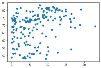
#scatterplot to of alcconsumption and lifeexpectancy
plt.scatter(data['alcconsumption'],data['lifeexpectancy']) plt.show()
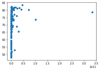
#scatterplot to of co2emissions and lifeexpectancy
plt.scatter(data['co2emissions'],data['lifeexpectancy']) plt.show()
Summary
Descriptive Statistics for alcconsumption Variable
count 172.000000
mean 6.631163
std 5.015301
min 0.030000
25% 2.390000
50% 5.865000
75% 9.810000
max 23.010000
Name: alcconsumption, dtype: float64
Frequency Distribution of alcconsumption
Counts
Low 77
Medium 54
High 41
Name: alcconsumptionrange, dtype: int64
Percentages
Low 0.447674
Medium 0.313953
High 0.238372
Name: alcconsumptionrange, dtype: float64
Desriptive Statistics for co2emissions Variable
count 172.000000
mean 5774913036.826859
std 27664356994.819237
min 850666.670000
25% 55778250.002500
50% 254030333.300000
75% 2319100666.750000
max 334000000000.000000
Name: co2emissions, dtype: float64
Descriptive Statistics for lifeexpectancy Variable
count 172.000000
mean 69.229465
std 9.803362
min 47.794000
25% 62.646000
50% 72.807000
75% 76.085500
max 83.394000
Name: lifeexpectancy, dtype: float64
Frequency Distribution of lifeexpectancy
Counts
Less than 50 8
70-80 79
50-60 29
Greater than 80 20
60-70 36
Name: lifeexpectancyrange, dtype: int64
Percentages
Less than 50 0.046512
70-80 0.459302
50-60 0.168605
Greater than 80 0.116279
60-70 0.209302
Name: lifeexpectancyrange, dtype: float64
Description
The three variables I have chosen, alcconsumption, co2emissions and lifeexpectancy, are all continuous variables. Therefore, in order to create frequency distributions for them I had to group the data for each variable. I did just that for two of the three variables. It was not done for co2emssions since the variable had such a wide range, grouping would have caused skewness. Instead of the frequency distribution, I did a descriptive statistics summary for co2emissions and the other two variables.
From creating these tables I first found that for the variable alcconsumption, most countries fell in the low category which is a reading under 5, then the second most fell in the medium category which is a reading of between 5 and 10 and the least prominent group was the high group which were countries with a reading over 10. The average reading was 6.63.
Second for co2emissions, I found that the highest emission was 334000000000 and the lowest was 850666.67. The mean was recorded at 5774913036.826859 and the median was 254030333.3. There were a few outliers that were significantly higher than the rest of the countries causing the stark difference between the mean and medium calculation.
Third for lifeexpectancy, I grouped them just like alcconsumption. This time into 5 categories; less than 50, 50-60, 60-70, 70-80 and greater than 80. The 70-80 category had the highest frequency, followed by 60-70, then 50-60, then greater than 80 ad finally less than 50.
The three variables above each had missing data and to deal with this, I removed rows with missing data. Since it was not that many rows, removing some kept the integrity of the dataset. Below you will find a couple scatter plots, plotting alcconsumpiton and co2emissions against lifeexpectancy. (ifeexpectancy on the x axis)
acconsumption vs lifeexpectancy
Co2emissions vs lifeexpectancy
0 notes
Text
Mastery Journey Timeline – Full Sail University
Jacob Starks
Mastery: Development and Leadership:
Goals:
1. Understand how I can use mastery concepts for personal development.
· To understand how I can use the mastery concepts I have learned, I will look for individuals who have mastered the concepts and create a similar model to applying these concepts.
2. Identify a master in my field.
· I will research a master in my field whom I can relate to.
3. Become a better academic researcher.
· I achieve this by relying on more than just my academic experience, as stated in Journal of Library Administration, “students’ strategies are influenced by both their non-academic search experiences as well as the broader academic context of their research tasks” (D'Couto, et al., 2015 pp. 562-576)
Foundations of Business Intelligence:
Goal:
1. Understand the core concepts and tools in business.
· To assist with understanding these core concepts, I will use tutorials found in Lynda such as: excel weekly tips, Tableau 10 Essential training. etc
2. Know what tool project managers use in BI systems.
· I will achieve this through content covered in class and other online resources
3. Know the difference in business and academic research methods.
· I learn this through understanding the industry. “It is imperative to understand industry needs - can be difficult if industry does not know what it wants as is often the case and do not understand the research process” (Prideaux, 2012)
Enterprise Data Management:
Goals:
1. Understand how businesses manage data.
· I will understand this by understanding Big Data and its changes. “Yet the biggest problem is not simply the sheer volume of data, but the fact that the type of data companies must deal with is changing” (Longbotton, 2011 pp. 11-12)
2. Know what enterprise systems support business processes.
· I will learn this through seeking out high demand companies and gathering information on what systems supports their business, also through class material.
3. Understand how to communicate/present complex technical information.
· I will overcome this goal through taking advantage of communicating and presenting opportunities in class and at work.
Business Intelligence Technologies:
Goals:
1. Understand the planning and management of data warehouse projects.
· I will understand this concept by know the current pains of data management. “Data warehousing efforts may not succeed for various reasons, but nothing is more certain to yield failure than lack of concern for the quality of the data.” (Ballou, et al., 1999).
2. Understand the architectural and physical design of data.
· I will learn these design types course material and reaching out to colleagues currently working with these design models.
3. Understand reporting, performance monitoring, and forecasting.
· Cultivating these skills with improved through opportunities in class.
Business Intelligence Analytics:
Goals:
1. Understand statistical and analytical techniques.
· Understanding these techniques will be done through course material.
2. Understand Bayesian paradigm and Bayesian statistical methods.
· I will use key points in the American Statistician understand these methods. “Basic concepts a student needs to understand Bayesian inference; Rare use of Bayesian methods in practice; Need for standards for Bayesian methods” (Moore, 1997 p. 254)
3. Critical thinking in the planning of BI and data warehouse projects.
· To achieve this goal, I will try to understand the difference in concepts that leads to good warehouse management strategies. “It is prudent at this point to delineate the difference between data, information, and knowledge” (Kimple, 2013 pp. 376-384)
Data Mining:
Goals:
1. Learn how to identify patterns in data.
· I will learn to identify patterns in data through analyzing data content in course material.
2. Understand data mining concepts.
· Understanding data mining concepts will come through online course resources like Udemy and Lynda.
3. Understand data mining-specific project management.
· I will use Software Magazine as a resource to achieve this goal, as an article discusses, “how various companies in United States use data mining in the business” (Wilson, 1997 p. S6)
Patterns and Recognition:
Goals:
1. Understand advanced data mining concepts and techniques
· I will learn these concepts through training and course material.
2. Understand the use of algorithms in BI systems.
· Understanding the use of algorithms in BI was found helpful in an academic research stating, “The algorithms used by BI software include regression analysis, naive bay, decision tree, association, and cluster analysis. By using association rules, it also creates a market basket analysis” (Chem, et al.)
3. Understand how algorithms are used in social network analysis.
· I will learn this concept through www.lynda.com network analysis tutorial.
Process and Modeling Analysis:
Goals:
1. Understand how BI systems are used to improve business processes.
· I will understand how BI improves business process by seeking training from my job’s BI Senior Analyst.
2. Understand practical applications of business-process analytics
· I understand these applications though studying and retaining course knowledge.
3. Understand statistical stimulation and modeling concepts.
· I will better understand this through creating trail models about how they are a reflection of each other as explained by Anu Maria, “Modeling is arguably the most important part of a simulation study. Indeed, a simulation study is as good as the simulation model” (Maria, 1997)
Data Visualization and Creative Reporting:
Goals:
1. Learn to present complex results to a wide range of audiences.
· I will learn to do this through opportunities throughout the course.
2. Understand tools used to create impactful visual data.
· I will understand these tool by engaging in Lynda courses.
3. Understand interfaces and web designs used for real-time data.
· I will understand by capitalizing on the limitations used to produce real-time data. “There are several limitations in existing systems for providing easy-to-access 3D visualization of the radar data to the user community” (Zhoa, 2008).
Business Intelligence Leadership & Communication Skills:
Goals:
1. Learn to listen, explain, and ask question surrounding complex information.
· I will learn this through attending online workshops and instructor live lectures.
2. Learn to match visualizations and infographics with texts.
· I will develop this skillset through reading and dissecting more infographic layouts. “infographics make a large amount of data more consumable, especially if the audience is new to the presented subject” (Mathematica Policy Research, 2016).
3. Learn legal issues that effects BI policy and implementations.
· I will use case studies to take a look at how legal issues effects BI
Business Intelligence Case Studies:
Goals:
1. Learn to apply practical applications of BI systems analytics to business problems.
· I will achieve this goal by learning and applying these applications through the course.
2. Use BI case studies to address real word problems.
· I achieve this goal by collecting case studies and relating them to how BI Analyst solve real problems
3. Become comfortable using virtual meeting, interviews, and presentation skills.
· I will continue to get well at this as I am currently using this tool and skills at my job.
Business Intelligence Capstone:
Goals:
1. Demonstrate mastery of program curriculum.
· I will do this presenting and well thought out and thesis and presentation.
2. Finish and present full thesis.
· I achieve this by studying great presenters, as stated in a Princeton article, “Take note of effective speaker and adopt their successful habits”. (Princeton, 2016)
3. Give final presentation with confidence and technical competence.
· I will do this out of preparation throughout the entire program.
Works Cited
A cautious approach to data mining [Journal] / auth. Wilson Linda. - [s.l.] : Bell Atlantic Corp, 1997. - 14 : Vol. 17.
An Analysis of Algorithms Used by Business Intelligence Software [Report] / auth. Chem Kuo Lane, Lee Huei and Shing Chen-Chi / Computer Informations Systems ; Eastern Michigan University .
Bayes for beginners? Some reasons to hesitate [Journal] / auth. Moore David S. // American Statistician. - [s.l.] : Taylor & Francis, 1997. - 3 : Vol. 51.
Big Data: Making sense of information [Journal] / auth. Longbotton Clive. - Newton : Tech Target, 2011. - 3 : Vol. 2.
Bridging the Gap Between Academic Research and Industry Research Needs [Report] / auth. Prideaux Professor Bruce / Cairns Campus ; James Cook University . - Queensland : James Cook University , 2012.
CRITICAL SUCCESS FACTORS FOR DATA WAREHOUSING: A CLASSIC ANSWER TO A MODERN QUESTION [Journal] / auth. Kimple James F. // Issues in Information Systems. - Moon Township : Robert Mooris University, 2013. - 1 : Vol. 14. - pp. 376-384.
Data Visualization and Infographis [Report] / auth. Mathematica Policy Research. - Princeton : Mathematica Policy Research, 2016.
Enhancing Data Quality In Data Warehous Environments [Journal] / auth. Ballou Donald P. and Tayi Giri Kumar. - [s.l.] : Pazer Information System, 1999. - 1 : Vol. 42. - pp. 73-78.
How Students Research: Implications for the Library and Faculty [Journal] / auth. D'Couto Michelle and Rosenhan Serena H. // Journal of Library Administration. - [s.l.] : Journal of Library Administration, October 2015. - 7 : Vol. 55. - pp. 562-576.
How to give a good presentation [Online] / auth. Princeton // Princeton. - 2016. - November 18, 2017. - https://www.princeton.edu/~archss/webpdfs08/BaharMartonosi.pdf.
INTRODUCTION TO MODELING AND SIMULATION [Report] / auth. Maria Anu. - Binghampton : State University of New York at Binghampton, 1997.
Real-time Data Delivery and Remote Visulaization through Multi-layer Interfaces [Conference] / auth. Zhoa Lan // Grid Computing Environments Workshop. - Austin : IEEE, 2008.
0 notes
Text
TensorFlow Basics
Computation Graph
If your aspirations are to define a neural net in Tensorflow, than your workflow would be to first construct the network by defining all computations. Each single computation adds a node to the so called Computation Graph. Providing data to a Session (will come to that later) will ask TensorFlow to executed the giving graph.
TensorFlow comes with a neat build in tool called the TensorFlow Graph visulaization that helps you to keep and insight in what computations is actually defined in a computation graph. A computation graph can get hairy very quickly as one adds many nodes to it, therefore the grpah visualization tool has been implemented which makes it faily easy to understand how the data flows to the graph at any given time.
Session Management
After the computation graph has been defined one has to take care of the Tensorflow Session Management. A Session is neccessary to execute the predefined computation graph. A node in a computation graph has no state before it is evaluated in a Session.
import tensorflow as tf a = tf.constant(1.0) b = tf.constatn(2.0) c = a * b print(c) #=> Tensor("mul:0", shape=(), dtype=float32) with tf.Session() as sess: print(sess.run(c)) print(c.eval()) #=> 30.0 #=> 30.0
The line c = a * b just describes how to Tensorflow constants should be manipulated without actually doing it. To run the computation, the note has to be evaluated in a Tensorflow Session. The same variable can have to completely different values in two different sessions (e.g depending on the specific input values ...).
To make life easy, especially when you are experimenting with Tensoflow in an iPython notebook, Tensorflow comes with the concept of an Interactive Session, which keeps the same Session open by default.This avoids having to keep a variable holding the session.
import tensorflow as tf sess = tf.InteractiveSession() a =tf.Variable(1) a.initializer.run() #No need to refer to sess print(a.eval()) #WORKS #=> 1
One important thing to keep in mind is: "A session may own resources, such as variables, queues, and readers. It is important to release these resources when they are no longer required. To do this, either invoke the close() method on the session, or use the session as a context manager."TF documentation
TensorFlow Variables
In TensorFlow there are two slighltly different concepts of variables. There a constants and variables. The big difference between those to options is that a constant does not neccessariliy be initialized while a variable must be.
Constants
import tensorflow as tf constant_zero = tf.constant(0) # constant with tf.Session() as sess: print(sess.run(constant_zero)) #=> WORKS
Variabels
"When you train a model, you use variables to hold and update parameters. Variables are in-memory buffers containing tensors. They must be explicitly initialized and can be saved to disk during and after training. You can later restore saved values to exercise or analyze the model." (TF documentation)
import tensorflow as tf constant_zero = tf.constant(0) # constant variable_zero = tf.Variable(0) # variable with tf.Session() as sess: print(sess.run(constant_zero)) #=> WORKS print(sess.run(variable_zero)) #=> ERROR! sess.run(tf.global_variables_initializer()) print(sess.run(variable_zero)) #=> WORKS
Note that a variable usually is defined by not only giving it a value but also a name:
variable_zero = tf.Variable(0, name="zero")
The name "zero" is the entity that the variable has been given in the Tensorflow namespace, while variable_zero is the local entity that the variable is being given in the python namespace. When referring to this variable in the Tensorflow computation graph one uses "zero", but on the other hand if one wants to print the variable in the python script one refers to it as variable_zero.
Feeds and Fetches
When a computation graph is defined, there are two different kinds of computations that can be performed on it: Feeds and Fetches. A Feed places data in to the computation graph while a Fetch extracts data from such.
The previously defined operations c.eval() as well as sess.run(c) are both TensorFlow Fetch operataions.
To input data into the computation graph one uses the very simple command called tf.convert_to_tensor():
import tensorflow as tf import numpy as np numpy_var = np.zeros((2,2)) tensor = tf.convert_to_tensor(numpy_var) with tf.Session() as sess: print(tensor.eval()) #=> [[ 0. 0.] # [ 0. 0.]]
It is not possible to evaluate a NumPy array in a Tensorflow session (AttributeError: 'numpy.ndarray' object has no attribute 'eval').
First the NumPy array has to be converted into a Tensorflow Tensor (which automatically creates a TF node that is inserted into the computation graph => Feed operation). The Tensor can the be evaluated in a Tensorflow session which in this case retuns [[ 0. 0.] [ 0. 0.]] as expected.
0 notes
Photo

Hey all, We are looking for an atleast 2 years of experience Fornt-end UI Designer. Salary negotiable for suitable candidates. Required urgently and for long term basis. Please send your resume to [email protected] or call at +91-9409394242 Fornt-end UI Designer (1 position) Experience: - 2-3 years of experience in Web applications design and development. - Excellent knowledge of Html, CSS, JavaScript, jquery, Bootstrap (all versions) - Excellent knowledge on data visulaization tool D3.JS - Working experience on React JS or Angular JS (version 2 and above) - Good knowledge of Client-Server Architecture, network communication and good designing principles. - Basic web and mobile apps design experience (UI elements, Icons etc.,) - Ability to write well-documented and maintainable JS code. - Familiarity with git - Test websites across multi-browser configurations and identify any issues - Strong interpersonal skills and demonstrated the ability to build professional relationships. - Excellent Problem solving skills with innovative and proactive approach. - Proficient in debugging and fixing bugs in minimal time - Ability to work individually and in a team. #frontenddeveloper #jobopenings #hiringnow #recruitment #vadodarahr #vadodara_lover #uideveloper — view on Instagram https://ift.tt/2NgasW1
0 notes
Text
Class 12 Homework 1: My Top CSS and JavaScript Data and Stats Visualization Libraries
1. Plotly https://plot.ly/
A powerful platform endorsed by NASA, Shell Global, Google. the intricacy of the different algorithms and how the chart is created is a bit overwhelming as a beginner.
2. Google Charts https://developers.google.com/chart/
Endless charts. Endless graphs. An active community. Endless updates!
3. Chart.js http://www.chartjs.org/
Open-source JavaScript chart. Love its simplistic but informative design. User Friendly. 8 ways to visulaize your data.
4. D3.js https://d3js.org/
From my reviews D3.js is one of the most popular platforms used. They rave about its flexablity and how if differentiate from normal graphic and data processing libraries.
5. dc.js https://dc-js.github.io/dc.js/
Open-source software. Neat little JavaScript lib with a great balance between visualization of the data and enabling the user to explore and test specific hypothesis.
6. Chartist.js https://gionkunz.github.io/chartist-js/
Great for graphic anamation and responsive charts. Popular pick.
0 notes
Photo

Murals and Math: One School's Solution to Graffiti - Ellie Balk wrote in Education, New York and News
The act of painting murals is empowering. Once a student makes a mark on a wall, it becomes his or hers. When you walk down the busy street of Graham Ave, almost every wall is covered in random tags. We help the students create public art that means something and has significance. Students living in Brooklyn need this kind of connection to their communities because when the students invest in their communities, the communities invest in them. These murals are also made for the neighborhood. The results are not only beautiful images, but also sparked conversations.
Continue reading on good.is
243 notes
·
View notes